pd-upic
pd-upic is a program developed in Pure Data that allows you to extract information from
svg files. SVGs are vector files commonly used for drawings and graphic design. What
pd-upic essentially does is, based on defined rules, place those drawings in time so they can
be “played” individually.
pd-upic?1) Install Pure Data.
2) Go to Help -> Find Externals and search for pd-neimog. Install the library.
3) Open a new Pure Data patch and create an object:
declare -lib neimog
4) To check if everything is set up correctly, create an object named
l.readsvg.
score?To create your first score, first download Inkscape (it’s free and open-source). After downloading and installing, the next step is to create a rectangle with a black stroke (outline). Note that in Inkscape, “stroke” refers to the outline of the shape, and “fill” refers to the inside of the shape. To set the stroke color in Inkscape, hold SHIFT and click a color; to set the fill color, just click a color.
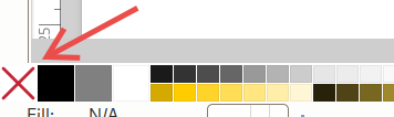
For pd-upic, this rectangle must have a black stroke and no fill. You can set no
fill by clicking the swatch that has an X in the center.
Below is an example of this rectangle:
Once the rectangle is created, right-click on its border and select Object Properties.
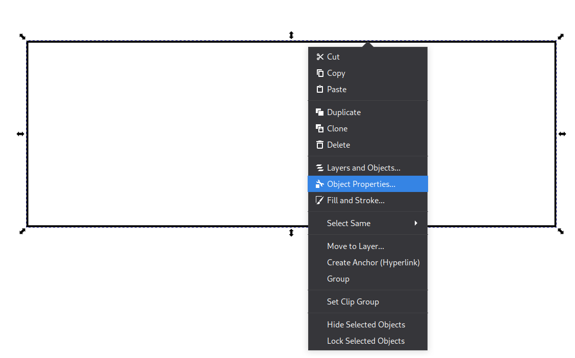
Everything inside this rectangle will be processed by pd-upic. Anything outside the rectangle will not be processed by pd-upic.
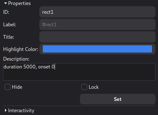
In the window that opens, you need to define two variables in the Description field:
onset and duration, specified in milliseconds. For example:
duration 5000, onset 0. In this case, this rectangle will start being played at millisecond 0
and end at millisecond 5000. After entering the variables, don’t forget to click Set—without
this, the variables will not be saved.
Once that’s done, anything you draw inside the rectangle will be processed by pd-upic. Anything outside will not be processed. You can use as many rectangles as you like; they will be processed individually.
In the drawing below, the red ellipse will be played very close to millisecond 0, the green ellipse around millisecond 2500, and the blue ellipse around millisecond 5000.
But you might wonder: what do I mean by “played”?
The svg file is read by a Pure Data object called l.readsvg. This object has two
main methods: read and play. The read method loads the
svg file you drew those objects in, so it requires you to specify the file’s location. In the
image below, I have an SVG file named simple-score in the same folder where this patch is saved.
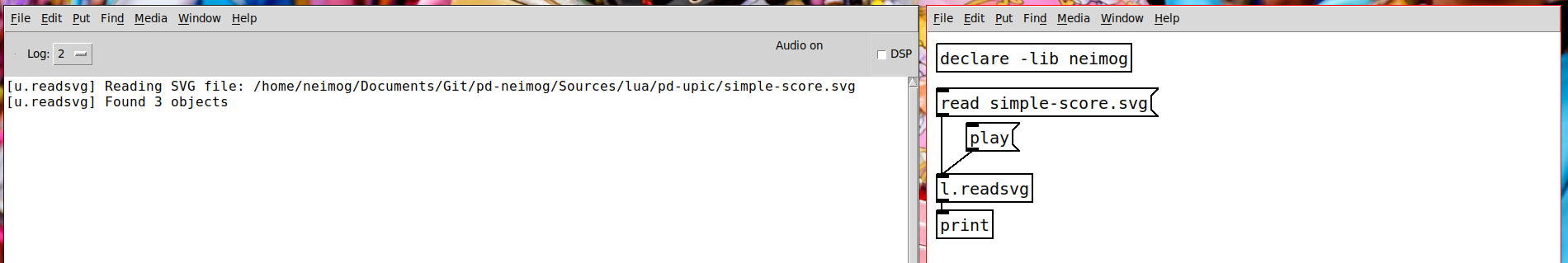
This file contains three playable objects: the red, green, and blue ellipses. When you press
play, the red ellipse will be played first, followed by the green and blue ellipses according
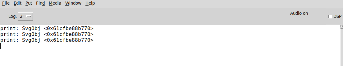
to their respective onsets. By “played,” I mean the moment when the ellipse is finally sent to the outlet of
the l.readsvg object.
From that outlet comes a message that may seem a bit odd at first. It should only be sent to
pd-upic objects or to objects that do not alter the message, such as triggers.
Okay, but now what do I do with this?
The idea is to route the information to specific subpatches, and inside those subpatches, extract the information and use it to create and synthesize sounds.
To filter drawings, you can use the l.attrfilter object. It works as follows: create the
object, provide the attribute you want to filter by, and then the value that attribute must have to
pass through the filter. For example, you can filter objects whose fill color is red using:
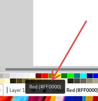
l.attrfilter fill #FF0000. If you’re not familiar with it, #FF0000 means
“red.” You can get this code in Inkscape by hovering the mouse over the selected color in the palette
(my screenshot tool doesn’t capture the cursor, but it was over the red square when I took the shot).
There are several parameters you can use as filters. Here’s a list of some of them:
| Attribute Name | Description | How to obtain |
|---|---|---|
fill |
The fill color of the drawing | Hover the mouse over the chosen color |
stroke |
The stroke (outline) color of the drawing | Hover the mouse over the chosen color |
relx |
Relative horizontal position (relative to the black rectangle), a number from 0 to 1; 0 is left and 1 is right. | Calculated based on where the drawing is relative to its parent |
rely |
Relative vertical position (relative to the black rectangle), a number from 0 to 1; 0 is bottom and 1 is top. | Calculated based on where the drawing is relative to its parent |
duration |
Object duration in milliseconds, based on how wide it is | Calculated from the drawing |
name |
The figure name, e.g., ellipse, circle, rect, among
others
|
Based on the SVG element used in the drawing |
You can always check the complete list using the l.attrprint object, which will print all
attribute names and their respective values.
Note that these objects only work with outputs from the pd-upic library.
Once you’ve filtered the objects, you can use their parameters musically. For example, we can use the
plaits~ object from the else library to play all objects that have a red fill.
This can be done using the patch below.
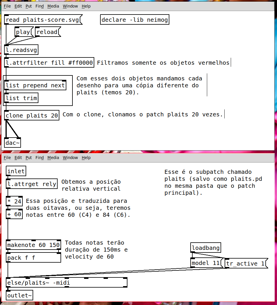
With this simple patch, we obtain the following result from the ‘score’ below.

All patches and examples are available in the folder neimog/lua/pd-upic, accessible
after installing the library—typically under Documents/Pd/externals/. In this example,
we could use the duration attribute to control the makenote duration, and use other
drawing parameters to control spatialization—there are many possibilities.